-
1) What is Geotechnical Numerical Analysis ?
-
2) Example & Conclusion
1. Concept of Geotechnical Numerical Analysis
In this lecture, We will learn about the concepts and principles of Geotechnical numerical analysis. we will learn about the Single degree of freedom system (SDOF) and multiple degrees of freedom system (MDOF). then, we will see in detail the procedure to perform numerical (FEM) analysis using the software. After that, we Analyse the 1D, 2D, and 3D models using GTS NX software.
Chapter 1) What Is Geotechnical Numerical Analysis?
- Introduction to Geotechnical numerical (FEM) analysis
- Stiffness formulation for a Single degree of freedom system (SDOF)
- Stiffness formulation for multiple degrees of freedom system (MDOF)
- procedure to perform numerical (FEM) analysis
Chapter 2) Example
- Modelling, boundary condition setting, applying load using Midas GTS NX software to 1D, 2D, and 3D models.
- Analysis and compare the results for the same.
Summary
The problems that need to be solved through geotechnical engineering are called geotechnical problems, and representative geotechnical problems include collapse, settlement, infiltration, and compaction.

The soil analysis methods that have been covered in soil mechanics or foundation engineering mainly correspond to theoretical analysis methods.
Also, in addition to theoretical approaches, there are methods based on numerical analysis, methods based on (model) testing, empirical methods, and others.
These analysis methods can be considered as tools for solving geotechnical problems, and here we will learn how to deal with geotechnical problems using numerical analysis methods.
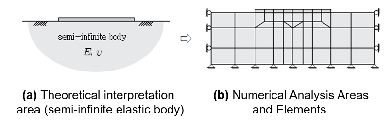
The representative numerical analysis method is the finite-element method (FEM), which is currently the most widely used numerical analysis method.
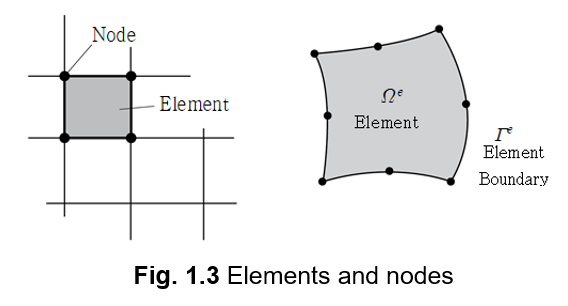
FEM divides the target problem into a finite number of elements (small regions) as shown in Figure 1.2, and uses the continuity at the nodal points of the elements to obtain nodal solutions instead of continuous solutions.
Each finite region is called an element, and the intersection of the lines that divide the elements is called a node (Figure 1.3).
The finite element method is a problem of solving a multivariate system of equations for nodal behavioral variables (unknowns), and the number of unknowns is roughly '(number of nodes) x (number of degrees of freedom at each node)’.
It follows principle that the closer is the size of the element is to zero, the closer is the obtained results to the theoretical solutions.
The solution method of numerical analysis is completely different from the traditional analytical methods, and the analysis is usually performed using commercial software.
We will cover an overview of numerical analysis from Lecture 1 to Lecture 3, so that you can learn it thoroughly.
Actual finite element analysis is performed using commercial software. (ex. midas GTS NX)
The general procedure of finite element analysis is as follows (★ denotes the area where engineers are involved)
(1) Modeling and meshing (★+SW)
Modeling is the process of selecting element types (number of nodes, shape functions) and inputting materials, among other things.
In general, the meshing process uses auto mesh generation of a computer to generate elements using basic data such as material, boundaries and geometric ranges.
(2) Element stiffness matrix calculation (SW)
For each model element, the stiffness matrix of each element is calculated. ( Ex. [K^e] {〖∆u〗^e} = {〖∆R〗^e} )
(3) Load and displacement boundary condition setting (★+SW)
When the engineer inputs the load, the software calculates the nodal load vector.
By inputting the nodal displacement conditions at the model boundary, the system equations are adjusted and the scale of the equations to be actually solved is determined.
(4) Composition of the overall system equation (SW)
Once the stiffness matrices of all elements have been obtained from the previous process, they must be assembled into a single system equation.
The equation to be solved is determined using the load and displacement boundary conditions.
(5) Solving the system equation(SW)
The system equation is expressed in the form of a multi-dimensional simultaneous equation.
First, the equation is solved to obtain the displacement at each nodal point, and then second-order calculations are used to calculate stress and strain from the displacement.
(6) Result Output (★+SW)
The engineer confirms the desired results in the form of numerical values, graphs, contour lines, color displays, and other program options.
As numerical analysis generally involves a huge amount of computation proportional to the number of elements and nodal points, the analysis process is divided into pre-processing, which involves preparing and inputting data, and post-processing, which involves visually processing the results, as shown in Figure 1.6.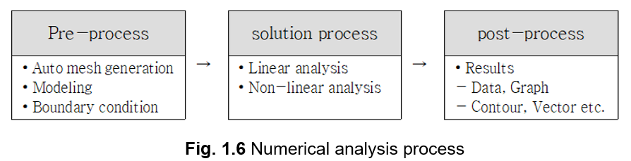
- MIDAS Members My profile Sign up

© MIDAS IT Co., Ltd.